import numpy as np
from patsy import dmatrix
import statsmodels.api as sm
import plotly.graph_objects as go
from numpy.linalg import inv
# generate data
np.random.seed(42)
x = np.random.uniform(0, 1, 50)
x = np.sort(x)
err = np.random.normal(0, 1, 50)
y = np.add(x, err)
# linear regression
def GLCov(x, sigma):
x_m = np.array([np.ones(len(x)), x]).transpose()
x_m_t = x_m.transpose()
x_c = np.matmul(x_m_t, x_m)
x_c_inv = inv(x_c)
x_c_inv = x_c_inv * (sigma * sigma)
return x_c_inv
cov = GLCov(x, 1)
pt_var = cov[0][0] + cov[1][1] * x * x + 2 * cov[0][1] * x
# global cubic
from numpy.linalg import inv
from numpy.linalg import multi_dot
def GlobalCubicCov(x, sigma):
x_m = np.array([np.ones(len(x)), x, x * x, x * x * x]).transpose()
x_m_t = x_m.transpose()
x_c = np.matmul(x_m_t, x_m)
x_c_inv = inv(x_c)
x_c_inv = x_c_inv * (sigma * sigma)
return x_c_inv
x_square = x * x
x_cubic = x * x * x
m = GlobalCubicCov(x, 1)
x_m = np.array([np.ones(len(x)), x, x * x, x * x * x]).transpose()
res = multi_dot([x_m, m, x_m.transpose()])
pt_var_cubic = res.diagonal()
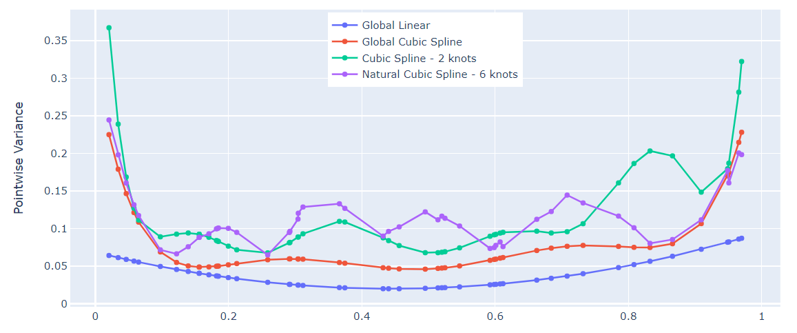
# Fit a cubic spline with two knots at 0.33 and 0.66
x_cubic = dmatrix('bs(x, knots=(0.33, 0.66))', {'x': x})
fit_cubic = sm.GLM(y, x_cubic).fit()
# Fit a natural spline with lower and upper bounds
x_natural = dmatrix('cr(x, df=6, lower_bound=0.1, upper_bound=0.9)', {'x': x})
fit_natural = sm.GLM(y, x_natural).fit()
# Create spline lines for 50 evenly spaced values of age
# line_cubic = fit_cubic.predict(dmatrix('bs(xp, knots=(0.33, 0.66))', {'xp': x}))
# line_natural = fit_natural.predict(dmatrix('cr(xp, df=6)', {'xp': x}))
# natural cubic spline
H = np.asarray(x_natural)
sigma = 1
m_Sigma = sigma * sigma * (inv(np.matmul(H.transpose(), H)))
m_cubic_natural = multi_dot([H, m_Sigma, H.transpose()])
res_cubic_natural = m_cubic_natural.diagonal()
# cubic spline
H = np.asarray(x_cubic)
sigma = 1
m_Sigma = sigma * sigma * (inv(np.matmul(H.transpose(), H)))
m_cubic = multi_dot([H, m_Sigma, H.transpose()])
res_cubic = m_cubic.diagonal()
# Create traces
fig = go.Figure()
fig.add_trace(go.Scatter(x=x, y=pt_var,
mode='lines+markers',
name='Global Linear'))
fig.add_trace(go.Scatter(x=x, y=pt_var_cubic,
mode='lines+markers',
name='Global Cubic Spline'))
fig.add_trace(go.Scatter(x=x, y=res_cubic,
mode='lines+markers', name='Cubic Spline - 2 knots'))
fig.add_trace(go.Scatter(x=x, y=res_cubic_natural,
mode='lines+markers', name='Natural Cubic Spline - 6 knots'))
fig.update_layout(
xaxis_title="x",
yaxis_title="Pointwise Variance",
)
fig.update_layout(legend=dict(
yanchor="top",
y=0.99,
xanchor="center",
x=0.5
))
fig.show()