Ex. 9.6
Ex. 9.6
Consider the ozone data of Figure 6.9.
(a) Fit an additive model to the cube root of ozone concentration as a function of temperature, wind speed, and radiation. Compare your results to those obtained via the trellis display in Figure 6.9.
(b) Fit trees, MARS, and PRIM to the same data, and compare the results to those found in (a) and in Figure 6.9.
Soln. 9.6
We include Figure 1 as an example (similar to Figure 6.9 in the text). It seems that, compared to three-dimensional smoothing example in Figure 6.9, fitted curves from GAM and MARS are more irregular, so does the one from the tree method.
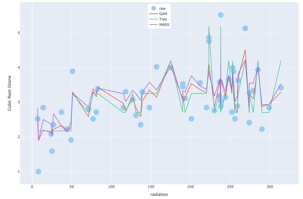
Figure 1: Ozone Data Example with GAM, Tree and MARS
Code
 1
 2
 3
 4
 5
 6
 7
 8
 9
10
11
12
13
14
15
16
17
18
19
20
21
22
23
24
25
26
27
28
29
30
31
32
33
34
35
36
37
38
39
40
41
42
43
44
45
46
47
48
49
50
51
52
53
54
55
56
57
58
59
60
61
62
63
64
65
66
67
68
69
70
71
72
73
74
75
76
77
78
79
80
81
82
83
84
85
86
87
88 | import pathlib
import numpy as np
import pandas as pd
import prim
from pyearth import Earth
from pygam import LinearGAM, s
from plotly.subplots import make_subplots
import plotly.graph_objects as go
from sklearn.tree import DecisionTreeRegressor
from sklearn.metrics import mean_squared_error
# get relative data folder
PATH = pathlib.Path(__file__).resolve().parents[1]
DATA_PATH = PATH.joinpath("data").resolve()
# ozone data
data = pd.read_csv(DATA_PATH.joinpath("ozone.csv"), header=0)
X = data.loc[:, 'radiation':'wind']
y = pd.DataFrame(data.loc[:, 'ozone'])
y['ozone'] = np.power((y['ozone']), 1 / 3)
# fit GAM
reg_gam = LinearGAM(s(0) + s(1) + s(2)).fit(X, y)
# reg_gam.summary()
y_pred_gam = reg_gam.predict(X)
print('MSE for GAM is {:.2f}'.format(mean_squared_error(y_pred_gam, y)))
# fit tree
reg_tree = DecisionTreeRegressor(max_leaf_nodes=5)
reg_tree.fit(X, y)
y_pred_tree = reg_tree.predict(X)
print('MSE for tree is {:.2f}'.format(mean_squared_error(y_pred_tree, y)))
# fit MARS
reg_mars = Earth()
reg_mars.fit(X, y)
# print(reg_mars.summary())
y_pred_mars = reg_mars.predict(X)
print('MSE for MARS is {:.2f}'.format(mean_squared_error(y_pred_mars, y)))
# plot 4 * 4
data_plot = X
data_plot['y'] = y
data_plot['y_pred_gam'] = y_pred_gam
data_plot['y_pred_mars'] = y_pred_mars
data_plot['y_pred_tree'] = y_pred_tree
data_pct = data_plot
data_pct = data_pct.sort_values('radiation')
data_pct = data_pct[data_pct['wind'] < data_pct['wind'].quantile(0.75)]
data_pct = data_pct[data_pct['temperature'] < data_pct['temperature'].quantile(0.75)]
# Create traces
fig = go.Figure()
fig.add_trace(go.Scatter(x=data_pct['radiation'], y=data_pct['y'],
mode='markers',
marker=dict(
color='LightSkyBlue',
size=20
),
name='raw'))
fig.add_trace(go.Scatter(x=data_pct['radiation'], y=data_pct['y_pred_gam'],
mode='lines',
name='GAM'))
fig.add_trace(go.Scatter(x=data_pct['radiation'], y=data_pct['y_pred_tree'],
mode='lines',
name='Tree'))
fig.add_trace(go.Scatter(x=data_pct['radiation'], y=data_pct['y_pred_mars'],
mode='lines',
name='MARS'))
fig.update_layout(
xaxis_title="radiation",
yaxis_title="Cubic Root Ozone",
)
fig.update_layout(legend=dict(
yanchor="top",
y=0.99,
xanchor="center",
x=0.5
))
fig.show()
|