Ex. 5.10

Ex. 5.10

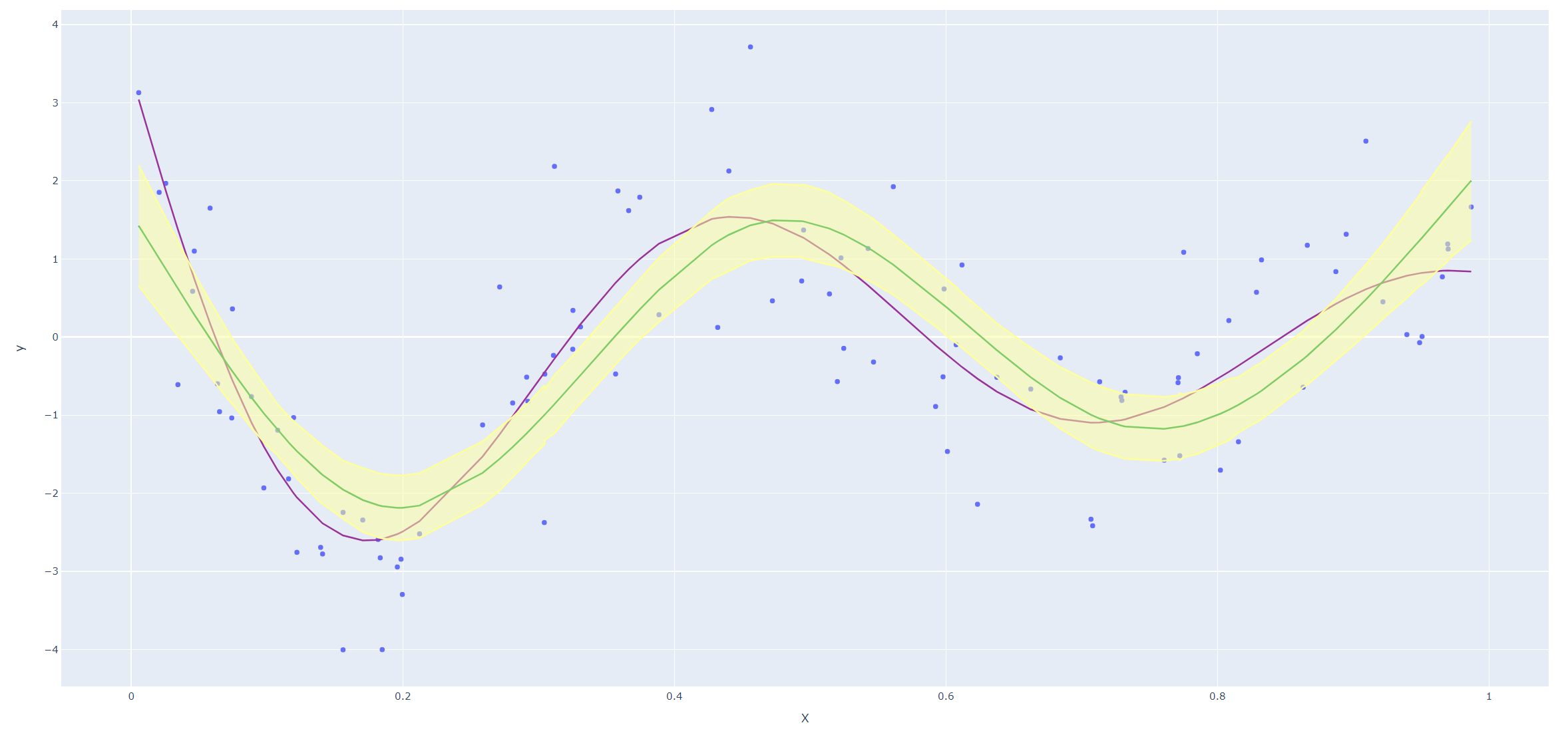
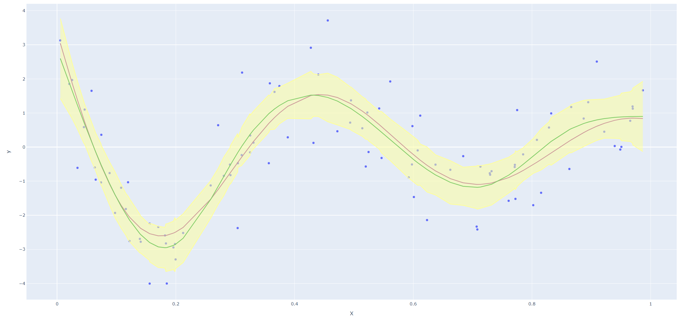
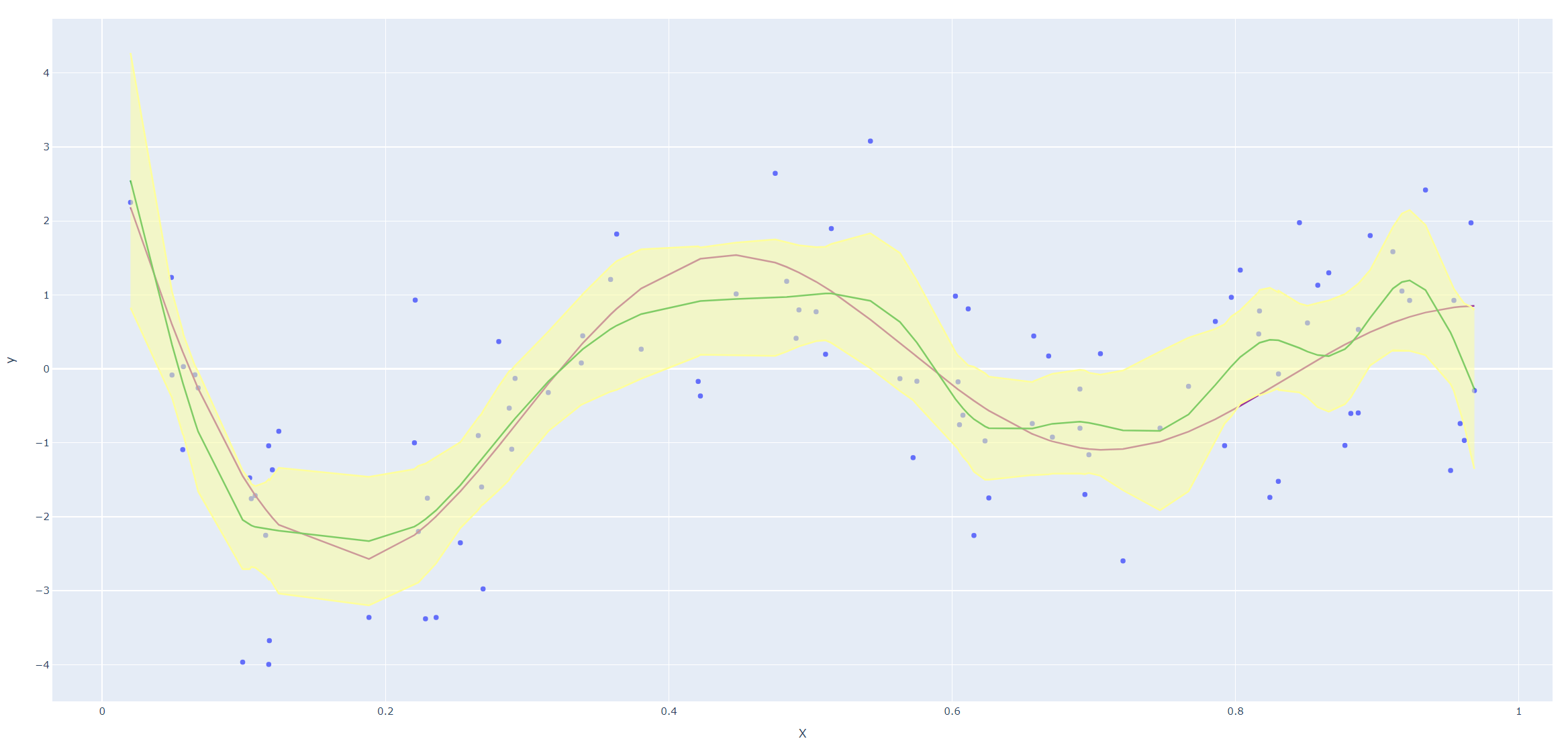
Derive an expression for \(\text{Var}(\hat f_\lambda(x_0))\) and \(\text{Bias}(\hat f_\lambda(x_0))\). Using the example (5.22), create a version of Figure 5.9 where the mean and several (pointwise) quantiles of \(\hat f_\lambda(x)\) are shown.

Soln. 5.10

Since

\[\begin{equation} \hat{\mathbf{f}} = \bb{N}(\bb{N}^T\bb{N} + \lambda \bm{\Omega}_N)^{-1}\bb{N}^T\by\non \end{equation}\]

we have

\[\begin{equation} \hat f_\lambda(x_0) = \bb{N}(x_0)^T(\bb{N}^T\bb{N} + \lambda \bm{\Omega}_N)^{-1}\bb{N}^T\by\non \end{equation}\]

where \(\bb{N}(x_0) = (N_1(x_0), ..., N_N(x_0))^T\). Therefore we have

\[\begin{eqnarray} \text{Var}(\hat f_\lambda(x_0)) &=& \bb{N}(x_0)^T(\bb{N}^T\bb{N} + \lambda \bm{\Omega}_N)^{-1}\bb{N}^T\text{Var}(\by)(\bb{N}^T\bb{N} + \lambda \bm{\Omega}_N)^{-1}\bb{N}(x_0)\non \end{eqnarray}\]

and

\[\begin{eqnarray} \text{Bias}(\hat f_\lambda(x_0)) &=& f_\lambda(x_0) - E[\hat f_\lambda(x_0)]\non\\ &=&f_\lambda(x_0) - \bb{N}(x_0)(\bb{N}^T\bb{N} + \lambda \bm{\Omega}_N)^{-1}\bb{N}^T\by.\non \end{eqnarray}\]

Next we reproduce Figure 5.9 in the text. Since smoothing splines has an explicit, finite-dimensional, unique minimizer which is a natural cubic spline with knots at the unique values of the \(x_i\), we could use codes for natural cubic splines (I haven't found a convenient package for smoothing splines in Python yet.)

Figure 1: df=5

Figure 2: df=9

Figure 3: df=15

Code
 1
 2
 3
 4
 5
 6
 7
 8
 9
10
11
12
13
14
15
16
17
18
19
20
21
22
23
24
25
26
27
28
29
30
31
32
33
34
35
36
37
38
39
40
41
42
43
44
45
46
47
48
49
50
51
52
53
54
55
56
57
58
59
60
61
62
import numpy as np
from numpy.linalg import multi_dot
import statsmodels.api as sm
from patsy import dmatrix
import plotly.graph_objects as go
from numpy.linalg import inv


np.random.seed(42)
n = 100
sigma = 1


def f(x):
    return np.sin(12 * (x + 0.2)) / (x + 0.2)


X = np.random.uniform(0, 1, n)
X = np.sort(X)
epsilon = np.random.normal(0, sigma, n)
y_true = f(X)
y_realized = y_true + epsilon

df = 15

x_nc = dmatrix('cr(x, df={})'.format(df), {'x': X}, return_type="dataframe")
fit_natural = sm.GLM(y_realized, x_nc).fit()
line_nc = fit_natural.predict(dmatrix('cr(xp, df={})'.format(df), {'xp': X}))

H = np.asarray(x_nc)
sigma = 1
m_Sigma = sigma * sigma * (inv(np.matmul(H.transpose(), H)))
m_nc = multi_dot([H, m_Sigma, H.transpose()])
pt_var_nc = m_nc.diagonal()
pt_std_nc = np.sqrt(pt_var_nc)
upper = line_nc + 2 * pt_std_nc
lower = line_nc - 2 * pt_std_nc

# Create traces
fig = go.Figure()
fig.add_trace(go.Scatter(x=X, y=y_realized,
                        mode='markers',
                        name='Raw'))
fig.add_trace(go.Scatter(x=X, y=y_true,
                        mode='lines',
                        name='True',
                        line_color='#993399'))
fig.add_trace(go.Scatter(x=X, y=line_nc,
                        mode='lines',
                        name='Fitted', line_color='#009933'))
fig.add_trace(go.Scatter(x=X, y=lower,
                        mode='lines',
                        name='Lower Limit', line_color='#ffff99'))
fig.add_trace(go.Scatter(x=X, y=upper,
                        mode='lines',
                        name='Upper Limit', fill='tonexty', line_color='#ffff99'))
fig.update_layout(
    xaxis_title="X",
    yaxis_title="y",
)

fig.show()